Predicting Laminar Flow Velocity Profile Using Physics-Informed Neural Networks (PINNs)

Introduction

A Physics-Informed Neural Network (PINN) is a powerful tool for predicting laminar flow velocity profiles within channels, essential for designing efficient thermal and fluid systems. While traditional CFD methods require complex meshing and high computational resources, PINNs integrate physical laws directly into neural networks, ensuring accurate and computationally efficient flow prediction.

What is a Physics-Informed Neural Network?

A PINN is an advanced deep learning technique that incorporates governing physics equations into neural network training. Unlike traditional machine learning models, PINNs ensure physically meaningful solutions by solving partial differential equations (PDEs) as part of the training process.

Objective of the Simulation Using PINN for Laminar Flow

The primary goal of this study was to apply a Physics-Informed Neural Network to predict the laminar flow velocity profile within a two-dimensional rectangular channel by:

• Implementing a neural network model trained using fundamental fluid mechanics laws.
• Ensuring compliance with physical boundary conditions.
• Evaluating PINNs as a viable alternative to conventional CFD simulations.

Key Parameters Used

• Channel dimensions: Length = 1 m, Height = 1 m
• Pressure difference driving the flow: ΔP = 1 Pa
• Fluid dynamic viscosity: μ = 0.1 Pa·s
• Laminar flow conditions ensured throughout the analysis

Simulation Procedure Overview

The simulation involved the following essential steps:

1. Data Preparation:
   Training data generated using uniformly distributed points across the channel height.
2. Neural Network Setup:
   A feedforward neural network with 3 hidden layers (20 neurons each) and tanh activation function.
3. Training:
   Model trained using Adam optimizer for 5000 epochs, minimizing errors via physical equations.
4. Evaluation and Visualization:
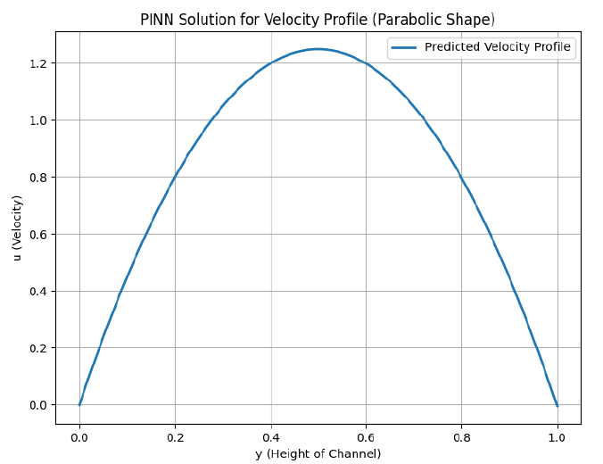
   The trained PINN accurately predicted a parabolic laminar velocity profile, matching theoretical expectations.

Results

The trained PINN model successfully captured the expected laminar velocity profile, demonstrating both high accuracy and computational efficiency. The predicted profile matched well-known theoretical results, validating the effectiveness of this approach.

Benefits of Using PINNs

• Lower Computational Costs – No need for complex meshing.
• Higher Accuracy – Physical constraints embedded in the model.
• Scalability – Extendable to complex fluid dynamics applications.

Complete Python Code for Simulation

Below is the complete Python implementation of the Physics-Informed Neural Network used in this simulation:

pythonCopyEditimport tensorflow as tf
import numpy as np
import matplotlib.pyplot as plt

# Define parameters
DeltaP = 1.0  # Pressure difference (Pa)
mu = 0.1      # Dynamic viscosity (Pa.s)
L = 1.0       # Channel length (m)
H = 1.0       # Channel height (m)

# Generate training data
N_points = 100
y_train = np.linspace(0, H, N_points).reshape(-1, 1)

# Define neural network (PINN)
class PINN(tf.keras.Model):
    def __init__(self):
        super(PINN, self).__init__()
        self.hidden_layers = [
            tf.keras.layers.Dense(20, activation='tanh') for _ in range(3)
        ]
        self.output_layer = tf.keras.layers.Dense(1)

    def call(self, y):
        x = y
        for layer in self.hidden_layers:
            x = layer(x)
        return self.output_layer(x)

# Loss function based on physics equations
def compute_loss(model, y_train):
    with tf.GradientTape(persistent=True) as tape:
        tape.watch(y_train)
        u_pred = model(y_train)
        du_dy = tape.gradient(u_pred, y_train)
        d2u_dy2 = tape.gradient(du_dy, y_train)

        residual = d2u_dy2 - DeltaP / (mu * L)
        residual_loss = tf.reduce_mean(tf.square(residual))

        # Boundary conditions: u=0 at y=0 and y=H
        u_0 = model(tf.constant([[0.0]], dtype=tf.float32))
        u_H = model(tf.constant([[H]], dtype=tf.float32))
        boundary_loss = tf.square(u_0) + tf.square(u_H)

        total_loss = residual_loss + boundary_loss
    return total_loss

# Single training step
@tf.function
def train_step(model, y_train, optimizer):
    with tf.GradientTape() as tape:
        loss = compute_loss(model, y_train)
    gradients = tape.gradient(loss, model.trainable_variables)
    optimizer.apply_gradients(zip(gradients, model.trainable_variables))
    return loss

# Initialize and train the model
model = PINN()
optimizer = tf.keras.optimizers.Adam(learning_rate=0.001)
epochs = 5000

for epoch in range(epochs):
    loss = train_step(model, tf.convert_to_tensor(y_train, dtype=tf.float32), optimizer)
    if epoch % 500 == 0:
        print(f"Epoch {epoch}, Loss: {loss.numpy()}")

# Predict and visualize results
y_test = np.linspace(0, H, 200).reshape(-1, 1)
u_pred = model.predict(y_test)

# Adjust velocity direction if needed
u_pred = -u_pred

plt.figure(figsize=(8, 6))
plt.plot(y_test, u_pred, label='Predicted Velocity Profile', linewidth=2)
plt.xlabel('Channel Height (y)')
plt.ylabel('Velocity (u)')
plt.title('Laminar Flow Velocity Profile Predicted by PINN')
plt.legend()
plt.grid(True)
plt.show()

Conclusion

Our study demonstrates that Physics-Informed Neural Networks (PINNs) provide an accurate, efficient, and practical alternative to traditional numerical methods for predicting laminar flow velocity profiles. By embedding the fundamental principles of fluid mechanics directly into neural network training, PINNs ensure physically consistent predictions while significantly reducing computational effort.

For an in-depth study, check our Articles.

More about PINNs on Wikipedia.